Convergence property for lp-l2 problem at the global minimizer

Posted June 23, 2011 by Lego
Categories: lp-l2 Optimization

For the following problem,

\text{min}~F(\mathbf{x})=\|\mathbf{A}\mathbf{x}-\mathbf{b}\|_2^2+\lambda \|\mathbf{x}\|_p^p,

we can prove that our algorithms proposed in PacRim 2011 and Asilomar 2011 have the following convergence fixed point property if the global minimizer \mathbf{x}^* is reached. Simply speaking, our algorithm assures that the next iterate will still be \mathbf{x}^*.

Let f(\mathbf{x})=\|\mathbf{A}\mathbf{x}-\mathbf{b}\|_2^2 and g(\mathbf{x})=\lambda \|\mathbf{x}\|_p^p.  Define

Q_L(\mathbf{x},\mathbf{y})=f(\mathbf{y})+\langle \mathbf{x}-\mathbf{y}, \nabla f(\mathbf{y}) \rangle + \dfrac{L}{2} \|\mathbf{x}-\mathbf{y}\|_2^2+\lambda \|\mathbf{x}\|_p^p

and

p_L(\mathbf{y})=\text{argmin}_{\mathbf{x}}~Q_L(\mathbf{x},\mathbf{y})

Theroem: If \mathbf{x}^*=\text{argmin}~F(\mathbf{x}), and \mathbf{z}^*=p_L(\mathbf{x}^*), then \mathbf{z}^*=\mathbf{x}^*

Proof:

With

f(\mathbf{x}) \leq f(\mathbf{y})+\langle \mathbf{x}-\mathbf{y}, \nabla f(\mathbf{y}) \rangle + \dfrac{L}{2} \|\mathbf{x}-\mathbf{y}\|_2^2,

we have

F(\mathbf{x}) \leq f(\mathbf{x}^*)+\langle \mathbf{x}-\mathbf{x}^*, \nabla f(\mathbf{x}^*) \rangle + \dfrac{L}{2} \|\mathbf{x}-\mathbf{x}^*\|_2^2+\lambda \|\mathbf{x}\|_p^p

=Q_L(\mathbf{x},\mathbf{x}^*).

Thus,

F(\mathbf{z}^*)\leq Q_L(\mathbf{z}^*,\mathbf{x}^*).

In addition, it is known that

Q_L(\mathbf{x},\mathbf{x}^*) \geq Q_L(\mathbf{z}^*,\mathbf{x}^*),

therefore,

F(\mathbf{z}^*) \leq Q_L(\mathbf{x},\mathbf{x}^*)

which yields

F(\mathbf{z}^*) \leq Q_L(\mathbf{x}^*,\mathbf{x}^*).

Besides,

F(\mathbf{x})\geq F(\mathbf{x}^*)=Q_L(\mathbf{x}^*,\mathbf{x}^*),

thus

F(\mathbf{z}^*)\geq Q_L(\mathbf{x}^*,\mathbf{x}^*).

In all it follows that

F(\mathbf{z}^*) = Q_L(\mathbf{x}^*,\mathbf{x}^*).

Thus,

\mathbf{z}^*=\mathbf{x}^*.

Convergence proof of our new algorithm for lp-l2 problem? (Part 2)

Posted May 5, 2011 by Lego
Categories: lp-l2 Optimization

The problem that follows is whether we can prove

Q_L(\mathbf{x},\mathbf{x}_n)-Q_L(\mathbf{x}_{n+1},\mathbf{x}_n)\geq \dfrac{L}{2} \|\mathbf{x}-\mathbf{x}_{n+1}\|^2

For notational simplicity, let \mathbf{u}:=\mathbf{x}_n and \mathbf{v}:=\mathbf{x}_{n+1}. It is known that

\mathbf{v}=\text{argmin}~\{\dfrac{L}{2} \|\mathbf{x}-(\mathbf{u}-\dfrac{1}{L}\nabla f(\mathbf{u}))\|_2^2+\lambda \|\mathbf{x}\|_p^p\}.

Let \mathbf{c}=\mathbf{u}-\dfrac{1}{L}\nabla f(\mathbf{u}). The previous inequality is equivalent to

\lambda \|\mathbf{x}\|_p^p- \lambda \|\mathbf{v}\|_p^p \geq \dfrac{L}{2} \|\mathbf{u}-\mathbf{v}\|^2+L \langle \mathbf{v}-\mathbf{x}, \mathbf{u}-\mathbf{c} \rangle

+\dfrac{L}{2}\|\mathbf{x}-\mathbf{v}\|^2-\dfrac{L}{2} \|\mathbf{x}-\mathbf{u}\|^2.

Therefore, if we can prove the inequality holds for each 1-D case, then the convergence proof is accomplished. By separation into a 1-D counterpart, the inequality we’d like to prove becomes

\lambda |x|^p-\lambda |v|^p \geq \dfrac{L}{2} (u-v)^2+L(v-x)(u-c)

+\dfrac{L}{2}(x-v)^2-\dfrac{L}{2}(x-u)^2,

which is found to be equivalent to

q(x)-q(v) \geq \dfrac{L}{2}(x-v)^2

where

q(s)=\dfrac{L}{2}(s-c)^2+\lambda |s|^p

and

v=\text{argmin}~q(s).

Based on our research conducted so far, it is hard (or not possible) to prove

q(x)-q(v) \geq \dfrac{L}{2}(x-v)^2

for 0<p<1. Though our simulations do show that the algorithm proposed in [2] converges, the convergence proof as well as the convergence rate is still an open question worthwhile to pursue.

[1] A. Beck and M. Teboulle, “A fast iterative shrinkage-thresholding algorithm for linear inverse problems,” SIAM Journal on Imaging Sciences, vol. 2, no. 1, pp. 183-202, 2009.

[2] J. Yan and W.-S. Lu, “New algorithms for sparse representation of discrete signals based on lp-l2 optimization,” submitted to PacRim 2011.

Convergence proof of our new algorithm for lp-l2 problem? (Part 1)

Posted May 4, 2011 by Lego
Categories: lp-l2 Optimization

In our recent paper [2], we investigate the lp-l2 problem with 0<p<1. Our algorithms are built on a recent algorithm known as the MFISTA [1], where a key step of soft shrinkage is replaced by a global solver for the minimization of a 1-D nonconvex problem.

It has been proved in [1] that for the l1-l2 problem, ISTA has a global convergence rate of O(1/k), and FISTA shares an improved complexity result of O(1/k^2). We naturally explore whether a similar convergence result exists for our algorithm reported in [2]. The lp-l2 problem considered is as follows

\text{min}~F(\mathbf{x})=\|\mathbf{A}\mathbf{x}-\mathbf{b}\|_2^2+\lambda \|\mathbf{x}\|_p^p.

Let f(\mathbf{x})=\|\mathbf{A}\mathbf{x}-\mathbf{b}\|_2^2 and g(\mathbf{x})=\lambda \|\mathbf{x}\|_p^p. The Lipschitz constant of the gradient \nabla f is L=2 \lambda_\text{max}(\mathbf{A}^T\mathbf{A}). It follows that

f(\mathbf{x}) \leq f(\mathbf{y})+\langle \mathbf{x}-\mathbf{y}, \nabla f(\mathbf{y}) \rangle + \dfrac{L}{2} \|\mathbf{x}-\mathbf{y}\|_2^2.

Thus,

F(\mathbf{x}) \leq f(\mathbf{y})+\langle \mathbf{x}-\mathbf{y}, \nabla f(\mathbf{y}) \rangle + \dfrac{L}{2} \|\mathbf{x}-\mathbf{y}\|_2^2+\lambda \|\mathbf{x}\|_p^p

=Q_L(\mathbf{x},\mathbf{y})

It can be derived that

Q_L(\mathbf{x},\mathbf{y})=\dfrac{L}{2} \|\mathbf{x}-(\mathbf{y}-\dfrac{1}{L}\nabla f(\mathbf{y}))\|_2^2+\lambda \|\mathbf{x}\|_p^p

+f(\mathbf{y})-\dfrac{1}{2L}\|\nabla f(\mathbf{y})\|_2^2

Suppose the current iterate is \mathbf{x}_n, and the next iterate is \mathbf{x}_{n+1}. By virtue of ISTA or FISTA (see [1]),

\mathbf{x}_{n+1}=\text{argmin}~\{Q_L(\mathbf{x},\mathbf{x}_{n}):~\mathbf{x} \in R^n\}

=\text{argmin}~\{\dfrac{L}{2} \|\mathbf{x}-(\mathbf{x}_n-\dfrac{1}{L}\nabla f(\mathbf{x}_n))\|_2^2+\lambda \|\mathbf{x}\|_p^p\}

It is not hard to derive that

F(\mathbf{x})-F(\mathbf{x}_{n+1}) \geq F(\mathbf{x})-Q_L(\mathbf{x}_{n+1},\mathbf{x}_n)

\geq f(\mathbf{x}_n)+\langle \mathbf{x}-\mathbf{x}_n,\nabla f(\mathbf{x}_n) \rangle + \lambda \|\mathbf{x}\|_p^p-Q_L(\mathbf{x}_{n+1},\mathbf{x}_n)

=\langle \mathbf{x}-\mathbf{x}_{n+1}, \nabla f(\mathbf{x}_n) \rangle + \lambda \|\mathbf{x}\|_p^p\lambda \|\mathbf{x}_{n+1}\|_p^p-\dfrac{L}{2}\|\mathbf{x}_{n+1}-\mathbf{x}_n\|_2^2

Therefore, if we can prove

\langle \mathbf{x}-\mathbf{x}_{n+1}, \nabla f(\mathbf{x}_n) \rangle+ \lambda \|\mathbf{x}\|_p^p-\lambda \|\mathbf{x}_{n+1}\|_p^p \geqL \langle \mathbf{x}_{n+1}-\mathbf{x}_n, \mathbf{x}_{n+1}-\mathbf{x}\rangle,

Then the following inequality holds

F(\mathbf{x})-F(\mathbf{x}_{n+1})\geq \dfrac{L}{2}\|\mathbf{x}_{n+1}-\mathbf{x}_n\|_2^2+L\langle \mathbf{x}_n-\mathbf{x},\mathbf{x}_{n+1}-\mathbf{x}_n \rangle

which essentially fits into the result of Lemma 2.3 in [1]. And if the inequality above holds, then the convergence proof for the lp-l2 problem follows in a same way as that of ISTA or FISTA for the l1-l2 problem.

At this point, the current problem is whether we can prove

\langle \mathbf{x}-\mathbf{x}_{n+1}, \nabla f(\mathbf{x}_n) \rangle+ \lambda \|\mathbf{x}\|_p^p-\lambda \|\mathbf{x}_{n+1}\|_p^p \geqL \langle \mathbf{x}_{n+1}-\mathbf{x}_n, \mathbf{x}_{n+1}-\mathbf{x}\rangle.

It can be calculated that this inequality holds if and only if

Q_L(\mathbf{x},\mathbf{x}_n)-Q_L(\mathbf{x}_{n+1},\mathbf{x}_n)\geq \dfrac{L}{2} \|\mathbf{x}-\mathbf{x}_{n+1}\|^2

[1] A. Beck and M. Teboulle, “A fast iterative shrinkage-thresholding algorithm for linear inverse problems,” SIAM Journal on Imaging Sciences, vol. 2, no. 1, pp. 183-202, 2009.

[2] J. Yan and W.-S. Lu, “New algorithms for sparse representation of discrete signals based on lp-l2 optimization,” submitted to PacRim 2011.

Homotopy Continuation for Sparse Signal Representation

Posted April 13, 2011 by Lego
Categories: lp-l2 Optimization

The \ell_1\ell_2 regularization problem, also known as basis pursuit (BP) is at the core of many signal processing applications and it has the following form

\text{min}~~~F(\mathbf{s};\lambda)=||\mathbf{y}-\mathbf{A}\mathbf{s}||^2+\lambda ||\mathbf{s}||_1

where the regularization parameter \lambda \geq 0 balances the tradeoff between sparsity and residual error. However, choosing the regularization parameter \lambda is a difficult task. A homotopy continuation-based method proposed in [1] is a algorithm that finds and traces all solutions \mathbf{s}^*(\lambda) as a function of the regularization parameter \lambda.

This algorihm allows one to solve the local problems (for a limited range of \lambda analytically, and piece together local solutions to get solutions for all regions of \lambda. The resulting algorithm generates solutions for all \lambda with a computational cost that is comparable to solving basis pursuit with quadratic programming for a single \lambda.

The implementation of the algorithm is quite involved. The fundamental basis is a non-smooth optimality conidtion for the convex function F. We describe the steps of the method in our report [2], and illustrate by a small example. Our simulations demonstrate the competence of the homotopy algorithm in finding \mathbf{s}^*(\lambda) for all \lambda when the problem involved is of a small scale. However, as the homotopy continuation algorithm requires computation of inverse of a matrix, we remark that for large-scale problems the matrix may be badly scaled. Thus, the stability of the homotopy algorithm is yet a practical issue that needs to be resolved.

For a clear and detailed description of the algorithm, please see the second part in my report [2].

[1] D. Malioutov, M. Cetin, and A. Willsky, “Homotopy continuation for sparse signal representation,” in Acoustics, Speech,and Signal Processing, 2005. Proceedings.(ICASSP’05). IEEE International Conference on, vol. 5. IEEE, 2005, pp. v–73

[2] ELEC 639A: “Fast Algorithms in Sparse Representations, Compressive Sensing, and Signal Denoising Based on lp-l2 Optimization; Homotopy Continuation Algorithms for l1-l2 Problems.” pdf

Isotropic and Anisotropic Total Variation From a Matrix Point of View

Posted April 12, 2011 by Lego
Categories: Uncategorized

Total variation (TV) proves to be an effective measure in the areas of image processing. We analyze the  TV in our technical report [1] from a matrix point of view. It is shown that the anisotropic TV can be equivalently computed by evaluating the l1 norm of a matrix-vector product,

\text{TV}_{\ell_1}(\mathbf{X}) =\|\mathbf{W}\mathbf{x}\|_{\ell_1}

where \mathbf{x} is generated by putting all the elements of \mathbf{X} column-wisely as a vector (implemented in MATLAB as x=X(:) ). The equation formulated above resembles the computation of the \ell_1 norm of wavelet coefficients of \mathbf{x}, under a wavelet transformation matrix \mathbf{W}. For an image \textbf{X} \in R^{M \times N}, however, we should note that matrix \textbf{W} is of size 2MN \times MN, which is not a square matrix. This is the fundamental difference between the total variation of an image \mathbf{X} and the \ell_1 norm of the wavelet coefficients of \mathbf{x} where the wavelet transformation matrix involved is square and most likely orthogonal if it is an orthogonal wavelet transformation.

Two MATLAB files in computing the isotropic TV and the anisotropic TV have also been prepared.

[1] J. Yan, Isotropic and Anisotropic Total Variation From a Matrix Point of View, Dept. of Electrical and Computer Engineering, University of Victoria, Victoria, BC, Canada, Apr. 2011. pdf code1 code2

Global Design of Perfect-Reconstruction Orthogonal Cosine-Modulated Filter Banks

Posted April 4, 2010 by Lego
Categories: Design of Digital Filters and Filter Banks


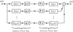
Orthogonal cosine-modulated (OCM) filter banks are among the most popular filter banks for multirate signal processing. The design of the prototype filter (PF) of an OCM filter bank can be expressed as

minimize e_2(\mathbf{h}) = \mathbf{h}^T \mathbf{P} \mathbf{h}

subject to:

a_{l,n}(\mathbf{h}) = \mathbf{h}^T \mathbf{Q}_{l,n} \mathbf{h} - c_n = 0
for 0 \leq n \leq m-1 and 0 \leq l \leq M/2-1

A great deal of research on (locally) optimal design of OCM filter banks has been made. However, their global design remains a challenge primarily because the design problem is nonconvex. The paper we published in [1] has proposed an order-recursive algorithm in achieving globally optimal design of OCM filter banks.

[1] J. Yan and W.-S. Lu, “Global design of perfect-reconstruction orthogonal cosine-modulated filter banks,” CCECE 2010, pp. 1-4, Calgary, AB, May 2009. pdf slides

Global Design of Orthogonal Filter Banks and Wavelets

Posted April 2, 2010 by Lego
Categories: Design of Digital Filters and Filter Banks

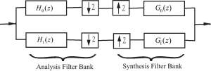
A two-channel CQ filter bank

Two-channel conjugate quadrature (CQ) filter banks are among the most popular building blocks for multirate syststems and wavelet-based coding systems, and have wide applications in general areas of digital signal processing. A two-channel CQ filter bank is required to satisfy the perfect reconstruction (PR) condition, and possibly to meet other constraints such as possessing certain number of vanishing moments (VMs). Generally, two design scenarios are considered, namely,

1. The least squares (LS) design

minimize \mathbf{h}^T \mathbf{Q} \mathbf{h}

subject to:

\sum_{n=0}^{N-1-2m} h_n \cdot h_{n+2m} = \delta_m for m=0,1,…,(N-2)/2

\sum_{n=0}^{N-1} (-1)^n \cdot n^l \cdot h_n = 0 for l=0,1,…,L-1

2. The minimax design

minimize \displaystyle{\mathop{\text{maximize}}_{\omega_a \leq \omega \leq \pi}}~|H_0(e^{j\omega})|

subject to:

\sum_{n=0}^{N-1-2m} h_n \cdot h_{n+2m} = \delta_m for m=0,1,…,(N-2)/2

\sum_{n=0}^{N-1} (-1)^n \cdot n^l \cdot  h_n = 0 for l=0,1,…,L-1

To date, only locally optimal design of CQ filter banks can be claimed. We have proposed strategies towards global designs of LS and minimax CQ filter banks. Several papers in this work have been published:

[1]  J. Yan and W.-S. Lu, “Towards global design of orthogonal filter banks and wavelets,” PacRim 2009, pp. 187-192, Victoria, BC, Aug 2009. pdf slides

[2] J. Yan and W.-S. Lu, “Towards global design of orthogonal filter banks and wavelets,” Canadian J. Elec. Comp. Eng., vol. 34, pp. 145-151, 2009. pdf

We have proposed another method which outperforms the above two papers for global designs of LS and minimax CQ filter banks.

Wavelet Transformation from a Matrix Point of View

Posted November 25, 2009 by Lego
Categories: Uncategorized

The filter bank structure of wavelet transformation is illustrated in the figure below. The input signal \mathbf{x} is a vector of length N, and we assume that N is a power of two. Based on this figure, wavelet decomposition is implemented through a series of filtering and downsampling processes.

A filter bank structure of wavelet transformation

We remark that wavelet transformation can be regarded as a matrix-vector multiplication from a linear algebra point of view, i.e., the wavelet coefficients \mathbf{y} of the input signal \mathbf{x} can be obtained through a matrix-vector multiplication \mathbf{y}=\mathbf{W} \mathbf{x}. The matrix \mathbf{W} is a mathematical representation of the filter bank structure and is called a wavelet matrix.

In our technical report [1], we present algorithms to formulate the wavelet matrix \mathbf{W}. The methods can be applied to both orthogonal and biorthogonal wavelet transformation and are of importance in areas such as compressive sensing, sparse signal processing and harmonic analysis.

The pdf version of the report, as well as the MATLAB mfile can be found at

http://www.ece.uvic.ca/~jyan/publications.htm

[1] J. Yan, Wavelet Matrix, Dept. of Electrical and Computer Engineering, University of Victoria, Victoria, BC, Canada, Nov. 2009. pdf code